Constructive Self-Supervised Learning (Part 1): Designing generalisable deep self-supervision, and predicting lower-level abstractions for better semantics.

Contents

• Introduction
• Principles for learning lower level abstractions (with deep self-supervision).
  • Setting a problem statement.
  • Predicting an abstraction hierarchy is a good (deep) objective.
• Why predicting a hierarchy is generally a good objective
  • What traditional SSL is doing
  • Why mainstream SSL converged on dispersion, and why that is limiting
• The Actual cI-JEPA Algorithm
  • Collected depths and teacher targets
  • Sampling source depths
  • Depth-specific predictor pathways
  • Multi-depth masked latent objective
  • Biasing supervision toward the deepest target
  • cI-JEPA summary
  • Evaluation methodology
  • Exact probe hyperparameters
  • Results and discussion
• Current SSL is probably doing some learning over the entire hierarchy of abstractions
• Some closing thoughts (on JEPAs)
• Acknowledgements
• References

Introduction

Traditionally, predicting lower-level abstractions is treated as harmful to learning higher-level semantics, and mainstream deep learning rarely supervises how intermediate abstractions are formed. This post argues for the opposite approach: we should explicitly shape the abstraction hierarchy during learning, and we should learn representations using signal from multiple levels of that hierarchy.

I call this family of objectives constructive SSL, because it explicitly supervises semantic construction. As a concrete example, I introduce cI-JEPA, a deeply supervised variant of I-JEPA¹ in which a small set of student depths predicts a hierarchy of teacher representations rather than a single final target. By changing how this hierarchy is weighted, we can control the tradeoff between retaining lower-level structure and composing toward higher-level abstractions.

On ImageNet-100 at ViT-B scale, this improves linear-probe accuracy over the I-JEPA baseline. More broadly, I will show two things: first, predicting an abstraction hierarchy is a useful way to design deep self-supervision for intermediate representations; second, using that same hierarchy to shape the final representation improves the final representation as well.

I perform my experiments on ImageNet-100 and ViT-B scale, and evaluate via improvement in linear probing accuracy on ImageNet-100.

The data and code can be found here. The code is designed to be run on a single 80GB A100/H100 on Google Colab.

Principles for learning lower level abstractions (with deep self-supervision).

Setting a problem statement.

Let’s assume we want to supervise semantic construction: shape intermediate abstractions as they form, not just the final representation. In modern deep nets, that usually means designing deep objectives that act on hidden representations.

A standard supervised deep loss, such as attaching a classifier to an intermediate layer², is poorly matched to this goal. It rewards whatever features solve the task immediately, including shortcuts, rather than abstractions that remain useful for later composition. That makes it a weak objective for shaping intermediate representations, especially on noisy natural data.

So for a given hidden representation, the deep objective should do two things: control the retention-dispersion tradeoff, and still bias learning toward higher-level composition. If there was sufficient communication bandwidth between the levels of abstraction (there isn’t in existing architectures), we wouldn’t have to keep all our building blocks in a single set of latents, and the purpose of deep supervision becomes largely to bias towards non-spurious higher-level composition.

Predicting an abstraction hierarchy is a good (deep) objective.

When representations are learned through prediction, the target level determines what the model is pushed to keep and compose. Higher-level targets bias learning toward composing higher-level abstractions, while lower-level targets bias learning toward retaining lower-level detail. Predicting a hierarchy, rather than a single level, therefore gives us a way to control this tradeoff across hidden representations.

A hierarchy target also makes shortcut solutions less attractive. If the loss only has to match one very high-level, low-bit target, spurious solutions can satisfy it more easily. Requiring a representation to explain multiple levels of abstraction imposes more semantic constraints, so the model is pushed toward compositions that remain useful across the hierarchy rather than for a single target alone.

This is still imperfect. Predicting lower-level targets is only an indirect way to preserve lower-level structure, and standard residual architectures are not efficient for routing across different levels of abstraction.

Predicting all the representations where all levels of abstraction are going to be learnt also provides conveniences for bootstrapping. For a given abstraction that we learn, the signal for learning it (i.e., the parts of the target hierarchy it’s supposed to be predicting) first forms dispersed throughout the network. We don’t know where exactly the ideal targets sit, and so we just predict everything. You will see concretely how this works in cI-JEPA.

Why predicting a hierarchy is generally a good objective

What traditional SSL is doing

Higher-level abstractions are usually more useful for downstream tasks than raw low-level detail. If the learning objective asks a model to predict very low-level targets such as pixels (see, MAE³), the model has to discover those higher-level abstractions indirectly. That is hard because the gap between the target and the abstractions we care about is large, and the resulting learning signal is noisy and sensitive to nuisance variation.

Latent SSL reduces this gap by predicting bootstrapped representations that are already biased toward higher-level structure rather than raw low-level targets. In effect, it lifts the level of abstraction at which supervision happens. Another way to describe this is that latent SSL works partly by dispersing lower-level detail. By not forcing the representation to preserve every low-level factor, it encourages the model to keep building blocks at a higher level of abstraction, which makes useful compositions easier to learn. The downside is that this mechanism is blunt with no controllability: it can also discard lower-level information that would still be useful for later composition or the final representation, and there are no knobs for us to use to tune how/what it discards.

Why mainstream SSL converged on dispersion, and why that is limiting

Mainstream latent SSL converged on dispersion largely because it lacks a direct way to encourage higher-level composition while still preserving useful lower-level detail. Dispersion is a shortcut: it suppresses low-level factors that are hard to compose and makes higher-level signals easier to learn. But it is also blunt. Some of the lower-level structure it throws away would still be useful for later composition or for the final representation, and it may not learn semantic compositions useful for more robust higher level abstractions. Further, predicting a representation where low level abstractions (e.g., chalk lines) are dispersed may throw away learning signals for learning some high level abstractions (e.g., math proof).

Constructive SSL is meant to replace that blunt tradeoff with explicit control over what gets retained, composed, and dispersed, while trying to learn more (lower level) semantic compositions for more robust higher level abstractions.

The Actual cI-JEPA Algorithm

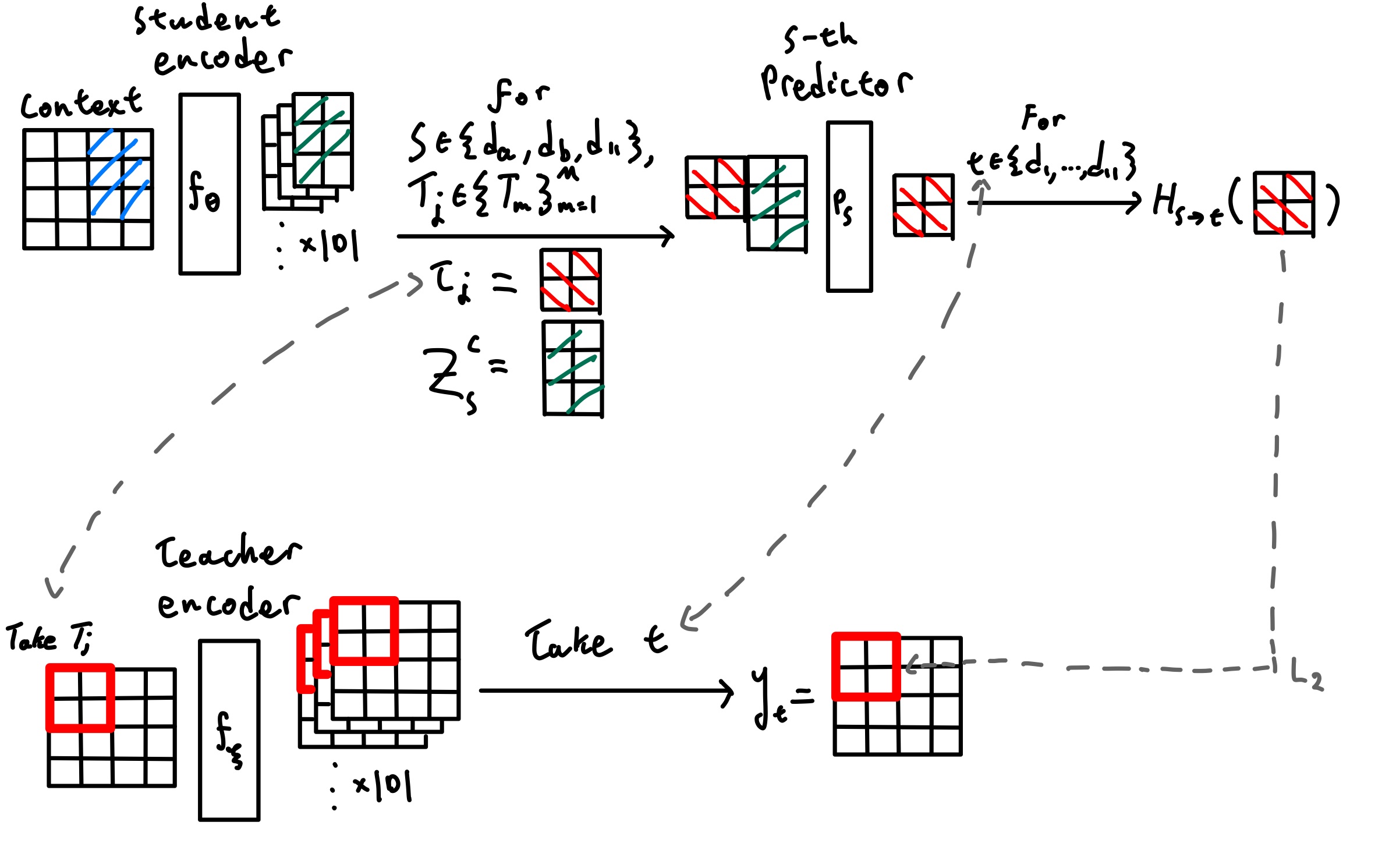cI-JEPA algorithm visual, based off of Figure 3 from I-JEPA paper¹.

I train a standard ViT-B/16. Relative to I-JEPA, the only substantive change is the objective: at each step, a small set of student depths predicts all collected teacher depths. Masking, target-location-conditioned prediction, and the EMA teacher essentially follow I-JEPA (though there are a few small implementation differences in masking).

In the scaled-down setting used here, I train on ImageNet-100 (about a tenth of ImageNet-1000 size) for 200 epochs by default, and always use a LR warmup covering roughly \(2.5\%\) of total training steps. cI-JEPA setup also removes the final encoder LayerNorm (done for consistency because there are no deep LayerNorms), uses constant weight decay \(0.05 \), as well as use RoPE instead of sincos positional embeddings (as more recent JEPAs use RoPE). The goal is to keep the optimization and masking recipe as close as possible to I-JEPA while changing only the supervision objective to minimize confounds.

Collected depths and teacher targets

Let the collected encoder depths be

In the experiments discussed here we use a ViT-B which has 12 transformer blocks, and unless otherwise noted we sample from the representations that come out of the deepest 11 blocks, so these are blocks \(1,\dots,11\). Note that \(d_{11}\) corresponds to the final output of the ViT-B.

The choice to not include the representation after the very first block in \(\mathcal D\) was accidental. I did not see a reason why this would affect the results or discussion so I didn’t re-run the experiments, but future work should probably include it (i.e., have \(\mathcal D = \{d_0, \dots, d_{11}\} \) ).

For an image \(x\), I sample context patches \(C\) and masked target blocks \(\{T_m\}_{m=1}^M\) exactly as in I-JEPA. The student encoder \(f_\theta\) only processes the context patches, while the EMA teacher \(f_\xi\) always processes the full image and provides stop-gradient targets:

where \(s,t \in \mathcal D\), \(f^{(s)}\) denotes the hidden state at collected depth \(s\), and \(\operatorname{sg}(\cdot)\) denotes stop-gradient.

Note that under standard I-JEPA with a ViT-B, the collected encoder depths are

Sampling source depths

A useful way to view cI-JEPA is as a source-depth \(\times\) target-depth table of prediction problems. Rows correspond to student source depths, and columns correspond to teacher target depths.

Unlike vanilla I-JEPA, cI-JEPA does not use all depths collected in \( \mathcal D \) as supervised rows at every step. Instead, I sample some number (two by default) of random intermediate rows and always include the deepest row:

So each optimization step supervises exactly three source depths: two random intermediate depths plus the final depth. Over training, all intermediate depths are revisited, but each step only pays for three source rows.

This sampling was mostly a training efficiency consideration. I did not ablate different choices for how many intermediate rows I sample each time during deep supervision due to compute constraints (this is a personal project), and always just sampled two when deep supervision is being done.

Depth-specific predictor pathways

Each sampled source depth \(s \in S\) has its own predictor pathway \(P_s\). Each predictor \(P_s\) is a separate instance of the narrow ViT that the I-JEPA uses.

It uses only the student context representation at that depth, together with the target block coordinates, to predict the masked block. In the implementation used here, these predictor pathways are fully separate rather than shared.

The predictor output is then mapped into each teacher depth with a bank of source–target-specific linear heads \(\{H_{s\to t}\}_{t\in\mathcal D}\):

The important point is that there is no fusion across source depths: each sampled depth must, by itself, predict the entire collected teacher hierarchy on the masked target block.

Multi-depth masked latent objective

The cI-JEPA objective is

where \(\ell\) is mean-squared error over the masked target tokens, and \(y_t^{\,T_m}\) denotes the teacher features at depth \(t\) for the target block \(T_m\).

In this setup, every sampled source depth predicts all target depths. The remaining design choice is therefore how to weight the target columns within each source row.

Biasing supervision toward the deepest target

Instead, I bias every row toward the deepest teacher target with all_to_last_weight, and I can further bias the final source row with last_to_last_weight.

Let

Then the row-wise target weights are

Because each row sums to one, these weights change where a row places its loss mass without changing the overall contribution of that row.

For example, when we have \(\alpha=0.5\) and \(\beta=0.8\) with \(L=11\):

• every non-final source row places \(50\%\) of its weight on the deepest teacher target and \(5\%\) on each of the other \(10\) depths;
• the final source row places \(80\%\) of its weight on the deepest teacher target and \(2\%\) on each of the other \(10\) depths.

Intuitively, this makes the deepest EMA representation the anchor of the objective. This deepest representation corresponds to the highest level of abstraction, and so by increasing \(\alpha, \beta\), you can bias the representations at a given source row towards higher level composition while still being grounded by the entire abstraction hierarchy by the residual loss.

As an implementation note, in the code, all_to_last_weight biases every source depth (including the last source depth) toward the last target depth, while last_to_last_weight only biases the last source depth toward the last target and leaves non-last source depths uniform. In the code, if last_to_last_weightis set, it will overwrite all_to_last_weight in the code.

cI-JEPA summary

One training step can be written as:

1. Sample masks as in I-JEPA.

   \[C,\; \{T_m\}_{m=1}^M \sim \text{MaskSampler}(x).\]

2. Sample the supervised source depths.

   \[S = \{d_a,d_b,d_{11}\}, \qquad d_a,d_b \sim \operatorname{Unif}(\mathcal D \setminus \{d_{11}\}), \qquad d_a \neq d_b.\]

3. Run the student on the context view only.

   \[\{z_s^C\}_{s\in\mathcal D} = f_\theta(x_C).\]

4. Run the EMA teacher on the full image.

   \[\{y_t\}_{t\in\mathcal D} = \operatorname{sg}\!\bigl(f_\xi(x)\bigr).\]

5. For each target block and each sampled source depth, predict the full teacher hierarchy.

   For every \(m \in \{1,\dots,M\}\), every \(s \in S\), and every \(t \in \mathcal D\),

   \[h_{s,m} = P_s(z_s^C, C, T_m), \qquad \hat y_{s\to t}^{\,T_m} = H_{s\to t}(h_{s,m}).\]

6. Accumulate the weighted multi-depth masked latent loss.

   \[\mathcal L_{\text{cI-JEPA}} = \frac{1}{M|S|} \sum_{m=1}^{M} \sum_{s\in S} \sum_{t\in\mathcal D} w_{s,t}\; \ell\!\left(\hat y_{s\to t}^{\,T_m},\, y_t^{\,T_m}\right).\]

7. Update the student, then update the EMA teacher.

   \[\theta \leftarrow \theta - \eta \nabla_\theta \mathcal L_{\text{cI-JEPA}}, \qquad \xi \leftarrow m\xi + (1-m)\theta.\]

Evaluation methodology

I evaluate frozen EMA teacher representations with a standard linear probe on mean-pooled final-layer patch tokens and report ImageNet-100 top-1 accuracy. Unlike the larger-budget linear probe used in the original I-JEPA work, I use a much smaller probe budget. The probe classifier is trained for only 10 epochs with batch size 256 using AdamW. The exact probe hyperparameters are listed below.

The data transforms follow the standard I-JEPA-style linear-evaluation recipe.

Exact probe hyperparameters

• Dataset: ImageNet-100
• Encoder used for probing: frozen EMA teacher encoder
• Representation: final-layer patch tokens, mean-pooled over spatial positions
• Probe head: single linear layer from embedding dimension to 100 classes
• Optimizer: AdamW
• Learning rate: 3e-3
• Weight decay: 0.0
• Epochs and LR schedule: linear decay from 3e-3 to 0.0 over 10 epochs
• Train batch size: 256
• Validation batch size: 256
• Probe train transform: RandomResizedCrop(224, scale=(0.08, 1.0), interpolation=BICUBIC) + RandomHorizontalFlip(0.5) + ImageNet normalization
• Probe validation transform: Resize(256, interpolation=BICUBIC) + CenterCrop(224) + ImageNet normalization
• Number of classes: 100

Results and discussion

Note that in the actual code, all_to_last_weight and last_to_last_weight don’t exactly correspond to \(\alpha\) and \(\beta\). In the code, if last_to_last_weight isn’t set, \(\beta\) will default to \(\alpha\).

The important observations:

1. R-A05-B10 beats both I-JEPA baselines, which suggests that hierarchy prediction is already useful as deep supervision even when the final representation predicts only the deepest target.

2. R-A05-B08 beats R-A05-B10, which suggests that asking the final representation to predict lower-level abstractions improves the final representation itself.

3. Weighting matters. Uniform supervision (R-U) under-composes, while overly strong deepest-target bias (R-A08-B08) hurts performance. The best result (R-A05-B08) uses moderate deepest-target bias in intermediate layers and stronger bias in the final layer.

4. R-B05 and R-B08 show that final-layer bias alone helps, but R-A.-B05 and R-A.-B08 show that final-layer hierarchy prediction without deep supervision is weak. The hierarchy becomes most useful when intermediate representations are also shaped.

5. As a sanity check, I also added the first block’s output (\(d_0\)) for run R-A05-B08-12. There’s a slight performance dip likely because predicting the first representation does not provide much learning signal.

Is this algorithm efficient? No. But I certainly hope it’s illustrative.

Current SSL is probably doing some learning over the entire hierarchy of abstractions

I think it’s also important to consider the possibility that current latent SSL methods are already somewhat learning over intermediate abstractions in the target, even if not explicitly doing deep supervision.

When people talk about “more pixel space information” vs “more semantic information” inside a representation, it’s useful to think of this as a weighted window on the spectrum of pixels to semantics, with higher absolute weighting on the spectrum meaning that the signals associated with that abstraction level are less dispersed/more easily recoverable from the representation (e.g., via a linear probe).

Through this writing, I often discretize this weighted window idea and refer to a single instance of an uneven weighted window as “a (single) level of abstraction”, even though it’s not entirely accurate. At any given “high-level” representation, we often retain some lower level abstractions.

Pixels are not linearly recoverable from SSL latents trained with I-JEPA or DINO⁴, but the RAE paper⁵ shows that you can recover pixels with a few (non-linear) tricks. This would be consistent with pixel-space information being dispersed in SSL latents. It likely also follows that intermediate abstractions are dispersed in SSL latents too, with the higher levels just being less dispersed. Using our weighted window analogy, current SSL representations have lower level abstractions less weighted, but still represent the entire hierarchy.

In DINO, the training target signal is bootstrapped from representations learned by the model itself. As said representations likely contain information about lower/intermediate abstractions, the target distribution likely does too (i.e., the target contains information about the entire abstraction hierarchy). Further, note that most modern neural nets have a residual connection, which is quite a natural bias towards retaining abstractions.

So, an interpretation of a factor behind the existing success of latent SSL may be that they already learn over the entire abstraction hierarchy.

It’s just that these lower level abstractions are worse and more dispersed, as their construction isn’t supervised, and we don’t provide some explicit target for them (and we can’t because they’re too dispersed).

Under constructive SSL, we learn better lower level compositions by supervising construction, and thus learn better lower level abstractions. This allows us to more explicitly specify a prediction objective over the entire abstraction hierarchy.

Some closing thoughts (on JEPAs)

Constructive SSL is a position about doing SSL. With current deep learning architectures, it will often use deep supervision; but I do not want to limit your imagination to doing deep supervision on existing architectures. The main intent of this blog post is an attempt at distilling the core ideas of what I think works for learning abstractions, not some more specific algorithm or implementation.

The choice of converting I-JEPA into cI-JEPA comes from the intuition that predicting representations directly provides the most “raw” signal for a given level of abstraction, and how they differ from other levels of abstraction. Further, working off of a well-known existing design makes the idea significantly more communicable, as well as provides a good baseline, to/for people.

Other choices like choosing instead to predict some distribution over prototypes like DINO may work, but they obscure the signal of the raw representation latents: DINO supervises a normalized prototype-assignment distribution (softmax outputs), which obscures information from the raw representation latents.

I also wouldn’t limit your imagination to doing just JEPAs. The important intuition that I’m trying to convey to you is simply that you should supervise the semantic construction of abstractions explicitly and learn by predicting varying levels of abstraction, and not just rely on an internal barely-constrained representation search while explicitly learning over a single level of abstraction (this applies to both methods like the MAE³ or I-JEPA).

Another intention of this design is to scale vision models. Scalable methods for intelligence have some notion of “more computing power can build/discover more abstractions from data”. Traditional latent SSL having a dispersion bias almost feels anti-scalable to me, as it throws away building blocks and potentially useful learning signals.

V-JEPA 2.1⁶ has a deep supervision setup that’s closest to cI-JEPA from what I am aware of. They fix the layers they’re supervising, as well as fuse the different intermediate representations by the channel for prediction, and predict many levels with a fused representation. I do think that the authors under-emphasised the interestingness of doing deep supervision. I think ideas I’ve presented are the factors that underlie why the V-JEPA 2.1 deep supervision works too.

I thought about calling my cI-JEPA design I-JEPA 1.1 because I think it’s a much more fitting name, but I did not want to impose a version number onto the original authors.

I would also not limit your imagination to vision or JEPAs. The idea behind doing representation learning more constructively is broadly applicable to everything. It is much more a way of thinking about how to learn good abstractions of reality than it is a specific vision (or even JEPA) thing.

I did not refer to constructive methods as JEPAs because it implies that you have to be predicting something, which may not always be the case. At least, you just want signals from the entire abstraction hierarchy that arises from nature, and explicitly shape the entire abstraction hierarchy. Though, it could turn out that all good constructive SSL objectives are JEPAs (i.e., you predict) anyways.

An original desire for this project was to find a way to represent an abstraction with the most efficient circuitry (least expressive power) possible. This and other ideas will hopefully be in part 2, where I talk a bit more about the interesting things you can do with a constructive objective.

Acknowledgements

Dominik and Minqi, and their LAPO paper⁷, was one of the initial inspirations for this project. When I was just starting out, Dominik said something to me like “just capture everything”. It was pretty nebulous to me what this meant at the time, but my current interpretation is something along the lines of “capture all the abstractions”.

Akarsh and Kenneth, their work on UFR/FER representations⁸ and evolutionary methods, as well as discussions we’ve had, helped shape and encourage some of these ideas.

Saining and Philip helped prompt some of these ideas.

Another initial inspiration of this project started out involving EBMs along with some guidance from Yilun⁹. I had (and have) a minor obsession with composing abstractions (with EBMs) which I couldn’t get working with existing methods, which led to this.

James, Samson, and Cem helped me pick out the naming scheme.

Cem and Leo (not his real name?) also read over this and suggested that I compact the text more. The version you see now is post-compaction.

References

M. Assran, Q. Duval, I. Misra, et al., “Self-Supervised Learning from Images with a Joint-Embedding Predictive Architecture,” arXiv:2301.08243, 2023. arXiv:2301.08243 ↩ ↩2
C.-Y. Lee, S. Xie, P. Gallagher, Z. Zhang, Z. Tu, “Deeply-Supervised Nets,” arXiv:1409.5185, 2014. arXiv:1409.5185 ↩
K. He, X. Chen, S. Xie, et al., “Masked Autoencoders Are Scalable Vision Learners,” arXiv:2111.06377, 2021. arXiv:2111.06377 ↩ ↩2
M. Caron, H. Touvron, I. Misra, et al., “Emerging Properties in Self-Supervised Vision Transformers,” arXiv:2104.14294, 2021. arXiv:2104.14294 ↩
B. Zheng, N. Ma, S. Tong, S. Xie, “Diffusion Transformers with Representation Autoencoders,” arXiv:2510.11690, 2025. arXiv:2510.11690 ↩
M. Assran, A. Bardes, D. Fan, et al., “V-JEPA 2: Self-Supervised Video Models Enable Understanding, Prediction and Planning,” arXiv:2506.09985, 2025. arXiv:2506.09985 ↩
D. Schmidt, M. Jiang, “Learning to Act without Actions,” arXiv:2312.10812, 2023. arXiv:2312.10812 ↩
A. Kumar, J. Clune, J. Lehman, K. O. Stanley, “Questioning Representational Optimism in Deep Learning: The Fractured Entangled Representation Hypothesis,” arXiv:2505.11581, 2025. arXiv:2505.11581 ↩
Y. Du, S. Li, I. Mordatch, “Compositional Visual Generation and Inference with Energy Based Models,” arXiv:2004.06030, 2020. arXiv:2004.06030 ↩